Code
# Get data
tuesdata <- tt_load('2024-09-24')
cty <- tuesdata$country_results_df
ind <- tuesdata$individual_results_df
time <- tuesdata$timeline_dfTidyTuesday Week 39
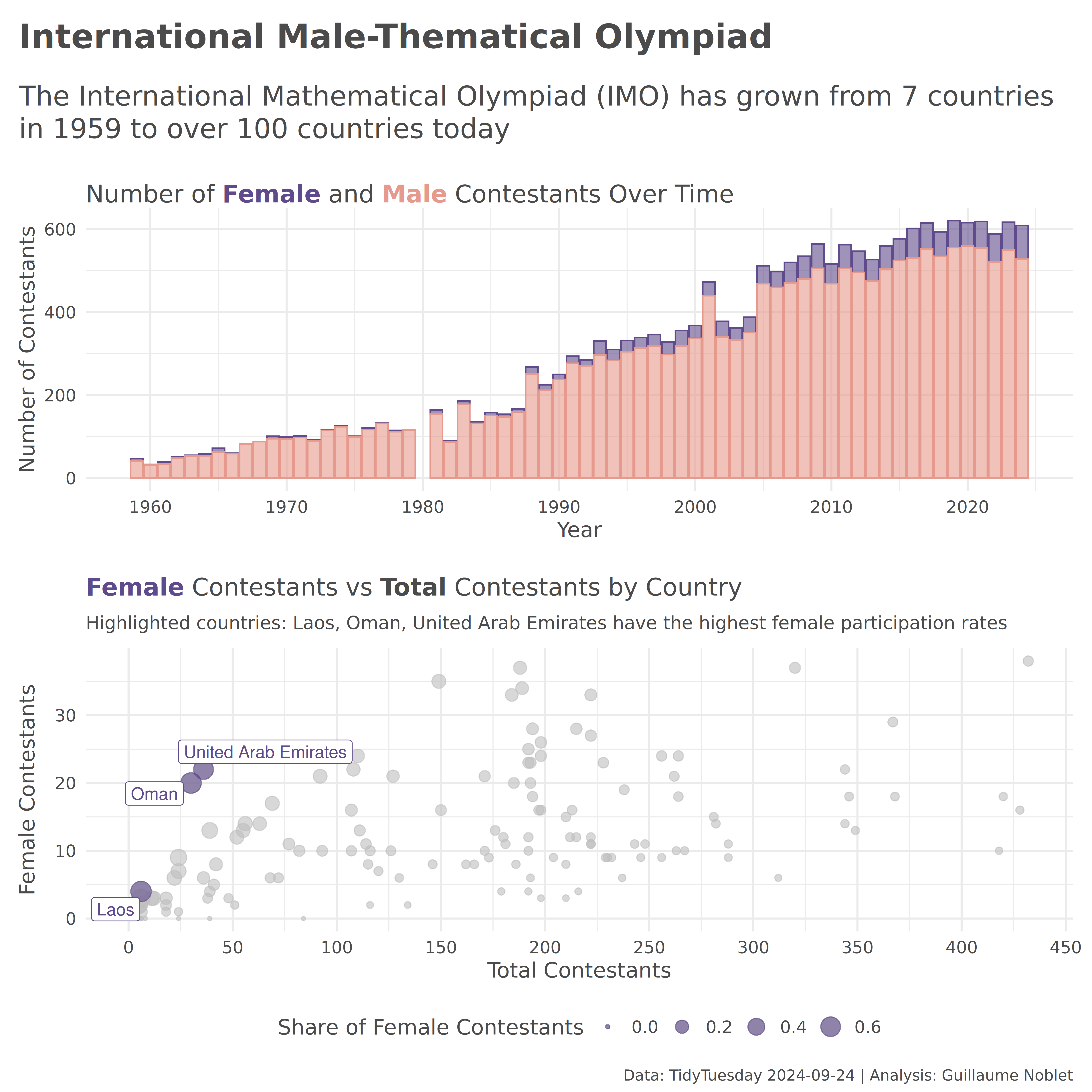
This week’s TidyTuesday explored the International Mathematical Olympiad (IMO) data, I look at gender participation patterns across countries and over time. The IMO is the World Championship Mathematics Competition for High School students, held annually since 1959.
The IMO dataset includes: - Country-level results and team compositions - Individual contestant results - Timeline data showing participation trends - Gender breakdown of contestants by country and year
# Get data
tuesdata <- tt_load('2024-09-24')
cty <- tuesdata$country_results_df
ind <- tuesdata$individual_results_df
time <- tuesdata$timeline_df# Prepare timeline data for gender analysis
time_longer <- time |>
tyr$pivot_longer(
cols = c(male_contestant, female_contestant, all_contestant),
names_to = "gender",
values_to = "n"
) |>
dyr$mutate(gender = sgr$str_remove(gender, "_contestant")) |>
dyr$select(year, country, countries, gender, n) |>
dyr$group_by(year, gender) |>
dyr$summarize(n = sum(n, na.rm = FALSE), .groups = "drop") |>
dyr$filter(gender != "all")# Analyze gender distribution by country
cty_gender_top_10 <- cty |>
dyr$group_by(country) |>
dyr$summarize(
tot = sum(team_size_all, na.rm = TRUE),
female = sum(team_size_female, na.rm = TRUE),
.groups = "drop"
) |>
dyr$mutate(share = female/tot)
# Get countries with highest female participation
cty_highest_share <- cty_gender_top_10 |>
dyr$arrange(dyr$desc(share)) |>
dyr$slice(1:3) |>
dyr$pull(country)
# Get countries with no female contestants
cty_no_female <- cty_gender_top_10 |>
dyr$filter(female == 0) |>
nrow()
cat("Countries with highest female participation:", paste(cty_highest_share, collapse = ", "), "\n")Countries with highest female participation: Laos, Oman, United Arab Emirates cat("Countries with no female contestants:", cty_no_female, "\n")Countries with no female contestants: 11 # Colors
female_col <- "#5F4B8BFF"
male_col <- "#E69A8DFF"
p1 <- gg$ggplot(time_longer) +
gg$geom_col(
gg$aes(x = year, y = n, color = gender, fill = gender),
alpha = 0.6
) +
gg$scale_color_manual(
values = c(female_col, male_col),
labels = c("Female", "Male")
) +
gg$scale_fill_manual(
values = c(female_col, male_col),
labels = c("Female", "Male")
) +
gg$labs(
x = "Year",
y = "Number of Contestants",
color = "Gender",
fill = "Gender",
title = "Number of <b><span style='color:#5F4B8BFF'>Female</span></b> and <span style='color:#E69A8DFF'><b>Male</b></span> Contestants Over Time"
) +
gg$scale_x_continuous(breaks = seq(1960, 2020, 10)) +
gg$theme_minimal(base_size = 14, base_family = "roboto") +
gg$theme(
plot.title = ggt$element_textbox_simple(size = 16),
legend.position = "none",
text = gg$element_text(family = "roboto", colour = "#4c4b4c")
)p2 <- gg$ggplot(cty_gender_top_10) +
gg$geom_point(
gg$aes(x = tot, y = female, size = share),
color = female_col,
alpha = 0.6
) +
ggh$gghighlight(
country %in% cty_highest_share,
label_key = country,
label_params = list(size = 4, color = female_col)
) +
gg$labs(
x = "Total Contestants",
y = "Female Contestants",
size = "Share of Female Contestants",
title = "<b><span style='color:#5F4B8BFF'>Female</span></b> Contestants vs <b>Total</b> Contestants by Country",
subtitle = paste("Highlighted countries:", paste(cty_highest_share, collapse = ", "), "have the highest female participation rates")
) +
gg$scale_x_continuous(breaks = seq(0, 500, 50)) +
gg$scale_y_continuous(breaks = seq(0, 100, 10)) +
gg$theme_minimal(base_size = 14, base_family = "roboto") +
gg$theme(
plot.title = ggt$element_textbox_simple(size = 16, margin = gg$margin(t = 10, b = 10)),
plot.subtitle = ggt$element_textbox_simple(size = 12, margin = gg$margin(b = 10)),
legend.position = "bottom",
text = gg$element_text(family = "roboto", colour = "#4c4b4c")
)# Create combined visualization
patchwork <- p1 / p2 +
pw$plot_annotation(
title = "<b>International Male-Thematical Olympiad</b>",
subtitle = "The International Mathematical Olympiad (IMO) has grown from 7 countries in 1959 to over 100 countries today",
caption = "Data: TidyTuesday 2024-09-24 | Analysis: Guillaume Noblet",
theme = gg$theme(
plot.title = ggt$element_textbox_simple(size = 22, margin = gg$margin(t = 10, b = 10)),
plot.subtitle = ggt$element_textbox_simple(size = 18, margin = gg$margin(t = 10, b = 20)),
plot.caption = gg$element_text(size = 10),
text = gg$element_text(family = "roboto", colour = "#4c4b4c")
)
)gg$ggsave('week_39.png', plot = patchwork, height = 10, width = 10, dpi = 600)gghighlight to emphasize countries with highest female participationpatchwork